 diamond_389.jpeg
Dark current and white field normalization
A simple-minded approach to reconstruction
Filtering before backprojection
This tutorial is intended to be a practical illustration of the steps involved in processing tomographic data. The tutorial uses actual data from a diamond crystal collected at the APS in April 1998. The computer code which implements each step in the processing is provided. The computer code is written in the IDL language, and is intended to serve as a model for C or C++ code which would be used for parallel processing version of these algorithms. Benchmark times are also given for each step in the processing, to give an idea of the relative computational costs of each processing step.
The data set in this example was collected in April 1998 on the GSECARS bending magnet beamline on Sector 13 at the APS. The sample is an opaque diamond, about 4 mm in diameter. The data were collected using monochromatic 10 keV x-rays. The sample radiographs were collecting using a single-crystal YAG scintillator placed 150 mm downstream of the sample. The visible light from the scintillator was imaged with a 5X Mitutoyo microscope objective onto a high-speed 12-bit CCD camera (Princeton Instruments Pentamax). The CCD has 1317x1035 pixels, each 6.7x6.7 microns. The field of view of the microscope was 4 mm, corresponding to 3 micron pixels on the YAG crystal and sample. The CCD readout was binned by a factor of 2 in each direction, resulting in a final pixel size on the sample of 6 microns. To minimize readout time and disk space a region-of-interest ROI of 658x342 binned pixels was defined around the sample image on the chip. Only this ROI was collected and stored at each point. The data collection was done using the EPICS scan record to drive the motor. The scan record communicated with a Visual Basic daemon on the PC via EPICS Channel Access. The daemon listens for requests to take an image, and then calls Princeton Instruments WinView via the Microsoft COM interface to take exposures and save them to disk.
The following computations were done using IDL 5.1 on a 300 MHz Pentium machine running Windows NT 4.0. The machine has 128MB of memory and 4 MB of SCSI disk.
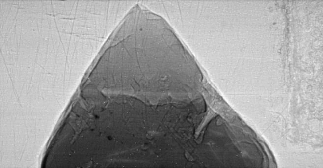
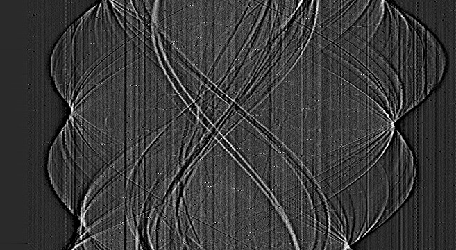
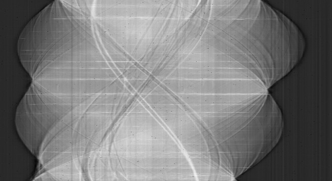
The raw data used for the microtomography were 12-bit images, each 658x342 pixels. The following is a typical image, displayed on a logarithmic intensity scale.
diamond_389.jpeg
A total of 360 such images were collected as the sample was rotated from 0 degrees to 179.5 degrees in 0.5 degree steps.
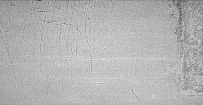
The first correction which must be applied to such images is for dark current and flat field. Dark current is the signal which is measured in the absence of any x-rays, and includes both true dark current (which is proportional to the exposure time), and the ADC pedestal or digitization offset, which is independent of exposure time. For the 10 second exposure times used in this experiment the true dark current was unmeasureable, while the pedestal was a very uniform 50�1ADC units per pixel. The white field is the image which is measured with the x-rays on, but without a sample in the beam. The non-uniformity in the white field includes effects of non-uniformities in the incident x-ray beam, non-uniform response of the scintillator and non-uniform response of the CCD detector. The following is a white field image collected just before the raw data image above, also displayed on a logarithmic intensity scale. Most of the defects in this white field image are due to scratches and contamination on the beryllium window at the end of the beamline.
 diamond_388.jpeg
The IDL code which computes the dark current and white-field corrected image is very simple:
; Tutorial1.pro
; This program reads in a raw image and a white field.  It stores them, plus the
; ratioed image as JPEG files
; The dark field of all of these images is a very uniform 50 counts
dark=50
read_princeton, '..\diamond389.SPE', raw_data
read_princeton, '..\diamond388.SPE', white_field
ratio = fix(10000 * float(raw_data-dark)/(white_field-dark))
; Write out images for Web page
t = bytscl(alog(raw_data))
write_jpeg, 'diamond_389.jpeg', rotate(t,-1), quality=90
t = bytscl(alog(white_field))
write_jpeg, 'diamond_388.jpeg', rotate(t,-1), quality=90
t = bytscl(alog(ratio))
write_jpeg, 'flat_field_corrected.jpeg', rotate(t,-1), quality=90
end
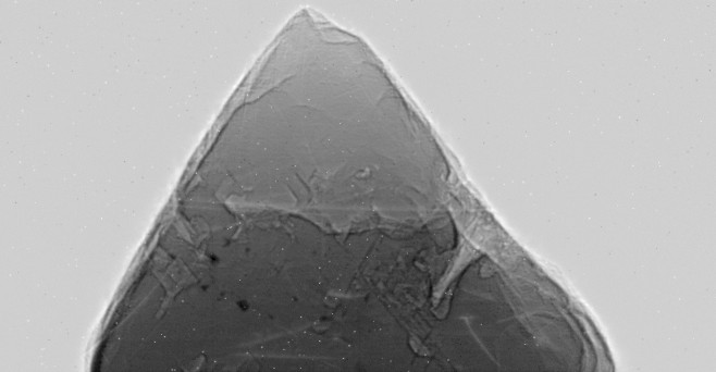
The ratio is converted to a 16-bit integer scaled by 10000 for efficiency. During the actual data processing the entire data volume, 658x342x360, is kept in memory. Using 16 bit integers results in an array size of 162 MB, while using a floating point array would use twice this much or 324 MB. The following is the image after correction for dark current and white field. Note that the intensity in the air outside the diamond is now very uniform, and the scratches are gone.
 flat_field_corrected.jpeg
The basic steps to reconstruct a slice through the object are as follows:
Here is is the IDL code which performs step 1 above:
; Program Tutorial1a.pro
; This program reads in the example diamond data.  It corrects for dark current and
; white field, and puts the data in a top-level IDL variable called volume
volume = intarr(658, 342, 360, /nozero)
data_files = strarr(360)
; The dark field of all of these images is a very uniform 50 counts
dark=50
; Read white field before and after
read_princeton, '..\diamond388.SPE', white1
read_princeton, '..\diamond570.SPE', white2
white = (float(white1-dark) + float(white2-dark))/2.
; Read first set of angles
for i=0, 179 do begin
	file =  '..\diamond' + strtrim((389 + i),2) + '.SPE'
	read_princeton, file, data
	volume[0,0,2*i] = 10000 * float(data-dark)/white
endfor
; Second set of angles
read_princeton, '..\diamond571.SPE', white1
read_princeton, '..\diamond754.SPE', white2
white = (float(white1-dark) + float(white2-dark))/2.
for i=0, 179 do begin
	file =  '..\diamond' + strtrim((573 + i),2) + '.SPE'
	read_princeton, file, data
	volume[0,0,(2*i)+1] = 10000 * float(data-dark)/white
endfor
end
Here is the code which implements steps 3-5 above:
; Program Tutorial2.pro
; This is a simple-minded approach to reconstructing a slice of the example diamond data
nangles = 360
angles = findgen(nangles)/(nangles-1) * !pi ; Evenly spaced angles 0 to 179.5 degrees
raw_sin = reform(volume[*,264,*])
corr_sin = sinogram(raw_sin, angles, air=20)
recon = backproject(corr_sin, angles)
; Write out images for Web page
t = bytscl(alog(raw_sin))
write_jpeg, 'sin1.jpeg', rotate(t,-1), quality=90
t = bytscl(corr_sin)
write_jpeg, 'sin2.jpeg', rotate(t,-1), quality=90
t = bytscl(-recon)
write_jpeg, 'recon2.jpeg', rotate(t,-1), quality=90
end
As called here, the sinogram code does the following:
-log(transmitted_intensity/air_intensity) at each point in each
row.The image above is the raw sinogram, before calling sinogram.
The image above is the corrected sinogram, after calling sinogram.
 recon2.jpeg
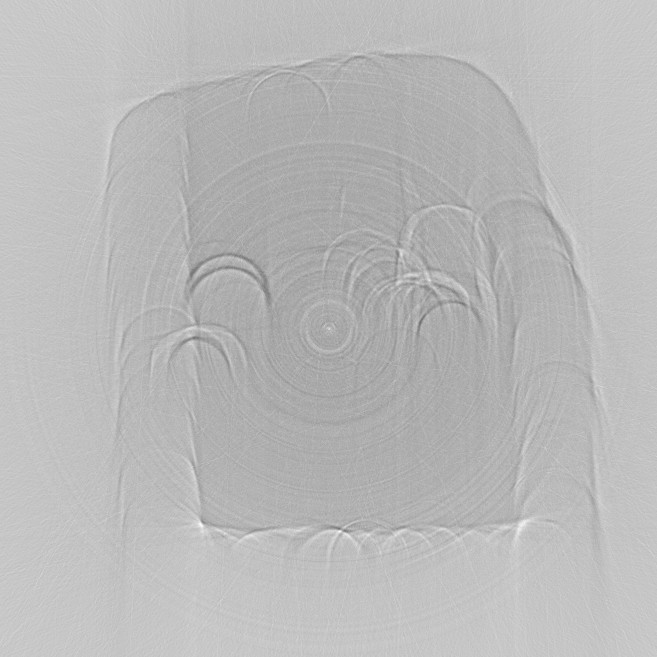
The image above is the reconstructed slice, after calling backproject.
The basic shape of the diamond is visible, but the reconstruction is very poor.
It is blurry, and dominated by artifacts. The following discussion outlines
the steps required improve this reconstruction by removing a variety of artifacts.
In the reconstruction above the backprojection was done without filtering the sinogram
first. This is main the reason why the reconstruction is so blurry. In
practice one always filters the sinogram before the backprojection. Here is a
modified version of the processing steps which includes a call to tomo_filter.
This results in a sinogram which is filtered using a Shepp-Logan filter, which is an
edge-sharpening filter.
; Program Tutorial3.pro
; This program filters the sinogram before backprojecting it
; It assumes that the volume array has already been read in
nangles = 360
angles = findgen(nangles)/(nangles-1) * !pi ; Evenly spaced angles 0 to 179.5 degrees
raw_sin = reform(volume[*,264,*])
corr_sin = sinogram(raw_sin, angles, air=20)
filtered_sin = tomo_filter(corr_sin, /shepp_logan)
recon = backproject(filtered_sin, angles)
; Write out images for Web page
t = bytscl(filtered_sin, min=-.01, max=.05)
write_jpeg, 'sin3.jpeg', rotate(t,-1), quality=90
t = bytscl(-recon, min=-10, max=2)
write_jpeg, 'recon3.jpeg', rotate(t,-1), quality=90
end
 sin3.jpeg
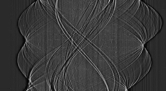
The image above is the filtered sinogram, after calling tomo_filter.
 recon3.jpeg
The image above is the reconstructed slice, after calling backproject with
the filtered sinogram. The image is much sharper than recon2.jpeg. The
dominant artifacts now are the downward curving arcs.
The reconstructions above were done without centering the sinogram on the rotation axis
before backprojecting. The poor centering is what causes the arc artifacts in
recon3.jpeg. Here is a modified version of the processing steps which includes the /center
option in the call to sinogram. This results in a sinogram which is
better centered on the rotation axis. sinogram does this centering by
determining the center-of-gravity of each row in the sinogram, and fitting this
center-of-gravity array to a sin wave. The symmetry axis of the fitted sin wave is
the rotation axis. The sinogram is then shifted left or right so that the rotation
axis is exactly on the center column of the sinogram array.
; Program Tutorial4.pro
; This program adds sinogram centering before filtering and backprojecting
; It assumes that the volume array has already been read in
nangles = 360
angles = findgen(nangles)/(nangles-1) * !pi ; Evenly spaced angles 0 to 179.5 degrees
raw_sin = reform(volume[*,264,*])
corr_sin = sinogram(raw_sin, angles, air=20, /center)
filtered_sin = tomo_filter(corr_sin, /shepp_logan)
recon = backproject(filtered_sin, angles)
; Write out images for Web page
t = bytscl(filtered_sin, min=-.01, max=.05)
write_jpeg, 'sin4.jpeg', rotate(t,-1), quality=90
t = bytscl(-recon, min=-10, max=2)
write_jpeg, 'recon4.jpeg', rotate(t,-1), quality=90
end
 sin4.jpeg
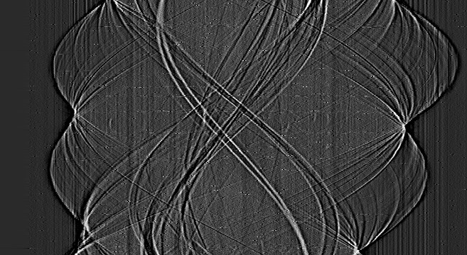
The image above is the centered sinogram, after calling sinogram with the /center
option. Note that it has been shifted to the right relative to sin3.jpeg.
 recon4.jpeg
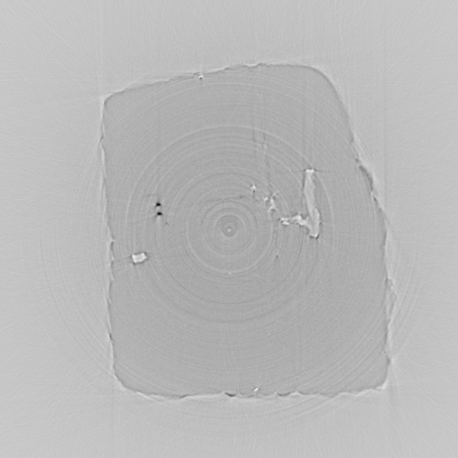
The image above is the reconstructed slice, after calling backproject with
the centered and filtered sinogram. The image is dramatically improved. Two
highly absorbing inclusions are clearly seen on the upper left, as well as voids or fluid
inclusions on the center left and right parts of the diamond. The dominant artifacts now
are the concentric rings.
The ring artifacts in the above reconstructions are due to drifts or non-linearities in the detector response. A bad detector element will show up as a vertical stripe in the sinogram, and there are clearly many such stripes in the sinogram sin4.jpeg. A vertical stripe on the sinogram backprojects as a half-cylinder centered on the rotation axis. The reason for this is clear, since a real object consisting of a thin cylinder centered on the rotation axis would appear as a two vertical lines in the sinogram. The causes of these vertical stripes in the sinogram can include the following:
I believe that most of the ring artifacts in these images are due to 3, harmonic contamination of the incident x-ray beam. The white field images are collected with no sample in the beam, and so are dominated by the fundamental energy, 10 keV in this case, from the Si [220] monochromator. However, the monochromator also passes the [440] at 20 keV, the [660] at 30 keV, etc. When the sample is placed in the beam the 10 keV photons are absorbed much more strongly than the 20 keV photons. If the ratio of 10/20 keV photons differs from one detector element to another, which can happen because of contamination of the Be window, defects in the monochromator, or defects in the scintillator, then different elements will have different response functions which are not removed by the flat-field correction.
Whatever their cause, the ring artifacts need to be suppressed to yield better reconstructions. The method I have used to reduce the ring artifacts is as follows:
The IDL procedure which implements this algorithm is remove_tomo_artifacts
with the /rings switch. Here is a modified version of the processing
steps which includes the call to remove_tomo_artifacts with the /rings
switch.
; Program Tutorial5.pro
; This program adds ring artifact reduction
; It assumes that the volume array has already been read in
nangles = 360
angles = findgen(nangles)/(nangles-1) * !pi ; Evenly spaced angles 0 to 179.5 degrees
raw_sin = reform(volume[*,264,*])
corr_sin = sinogram(raw_sin, angles, air=20, /center)
ring_sin = remove_tomo_artifacts(corr_sin, /rings)
filtered_sin = tomo_filter(ring_sin, /shepp_logan)
recon = backproject(filtered_sin, angles)
; Write out images for Web page
t = bytscl(filtered_sin, min=-.01, max=.05)
write_jpeg, 'sin5.jpeg', rotate(t,-1), quality=90
t = bytscl(-recon, min=-10, max=2)
write_jpeg, 'recon5.jpeg', rotate(t,-1), quality=90
end
 sin5.jpeg
The image above is the sinogram, after calling remove_tomo_artifacts with
the /rings option. Note that the vertical stripes have been
significantly reduced relative to sin4.jpeg.
 recon5.jpeg
The image above is the reconstructed slice, after calling remove_tomo_artifacts.
The ring artifacts have been significantly reduced relative to recon4.jpeg, without
noticeably changing the other parts of the reconstruction.
A close look at the 2 dark inclusions in the previous reconstruction, recon5.jpeg,
reveals that there is a bright streak extending down from the inclusions and a dark streak
extending up from them. These streaks are due to imperfect centering of the
sinogram. The automated sinogram centering
described above did not center the sinogram quite well enough in this case. The
reason is probably that these images contained diffraction artifacts (discussed elsewhere) which lead to the dark horizontal stripes in
the sinogram shown in sin1.jpeg. The dark stripes do
not affect the backprojection reconstruction significantly, but they do skew the
center-of-gravity calculation of the rotation axis center in sinogram.
In order to improve the centering I manually tweaked the sinogram centering using the tweak_center
keyword to sinogram until the resulting reconstruction had no streaks
above or below the high-contrast inclusions. Here is a modified version of the
processing steps which includes the call to sinogram with the tweak_center
switch. The center is tweaked by -2 pixels, or 12 microns in the negative direction.
; Program Tutorial6.pro
; This program adds sinogram center tweaking
; It assumes that the volume array has already been read in
nangles = 360
angles = findgen(nangles)/(nangles-1) * !pi ; Evenly spaced angles 0 to 179.5 degrees
raw_sin = reform(volume[*,264,*])
corr_sin = sinogram(raw_sin, angles, air=20, /center, tweak=-2)
ring_sin = remove_tomo_artifacts(corr_sin, /rings)
filtered_sin = tomo_filter(ring_sin, /shepp_logan)
recon = backproject(filtered_sin, angles)
; Write out images for Web page
t = bytscl(filtered_sin, min=-.01, max=.05)
write_jpeg, 'sin6.jpeg', rotate(t,-1), quality=90
t = bytscl(-recon, min=-10, max=2)
write_jpeg, 'recon6.jpeg', rotate(t,-1), quality=90
end
 sin6.jpeg
The image above is the sinogram, after calling sinogram with the tweak=-2
option. It is not perceptively different from sin5.jpeg above.
 recon6.jpeg
The image above is the reconstructed slice, after calling sinogram with
the tweak=-2 option. The streaks above and below the dark
inclusions, which were present in recon5.jpeg, are now gone.
A close look at recon6.jpeg above reveals perfectly straight, bright lines at random orientations in the image. These bright lines, which look like scratches, are due to zingers, or anomalously bright pixels, in the raw images. These zingers are caused by cosmic rays or scattered x-rays hitting the CCD chip directly, causing large energy deposition relative to the visible light photons from the scintillator crystal. The bright pixels in the images backproject as bright streaks, because they are equivalent to "tunnels" through the object which transmit x-rays only at one angle. Eliminating these zingers is best done when the raw data and white field images are first read in. The method I have used for zinger removal is the following:
The above algorithm is implemented in remove_tomo_artifacts with the /zingers
option. The following is the code which was used to read in the data for this sample
for the final reconstructions. This code reads in all of the files, corrects for
dark current, white field and zingers. It then writes the 3-D volume data back out
to disk at scaled 16 bit integers so that it can be read back into IDL for further
processing quickly, without having to read the individual data files again.
; This program reads all of the files for the large opaque crystal (diamond387-754.spe)
; and creates the 3-D file

pro read_data, file, data
    print, 'Reading file', file
    read_princeton, file, data
    data = remove_tomo_artifacts(data, /zingers, threshold=1.2)
end

; Main program
; Read one file to get the dimensions
read_data, 'diamond387.spe', data
size = size(data)
ncols = size[1]
nrows = size[2]

volume = intarr(ncols, nrows, 360, /nozero)
data_files = strarr(360)

; The dark field of all of these images is a very uniform 50 counts
dark=50

; Read white field before and after
read_data, 'diamond388.SPE', white1
read_data, 'diamond570.SPE', white2
white = (float(white1-dark) + float(white2-dark))/2.

; Read first set of angles
for i=0, 179 do begin
    file = 'diamond' + strtrim((389 + i),2) + '.SPE'
    read_data, file, data
    volume[0,0,2*i] = 10000 * float(data-dark)/white
endfor

; Second set of angles
; Read white fields before NONE after
read_data, 'diamond571.SPE', white1
read_data, 'diamond754.SPE', white2
white = (float(white1-dark) + float(white2-dark))/2.

; Read second set of angles
for i=0, 179 do begin
    file = 'diamond' + strtrim((573 + i),2) + '.SPE'
    read_data, file, data
    volume[0,0,(2*i)+1] = 10000 * float(data-dark)/white
endfor

print, 'Writing volume file ...'
write_tomo_volume, 'diamond_2.volume', volume
print, 'Done!'
end
sin7.jpeg
recon7.jpeg
The following code shows how the images for the Web page on the preliminary results on diamonds were produced. This is the top-level IDL program:
; This program writes the JPEG images for the diamond Web page

; Diamond 2
volume = read_tomo_volume('diamond_2.volume')
t = bytscl(alog(volume[*,*,0]))
write_jpeg, 'diamond_2_view0.jpeg', rotate(t,-1), quality=90
t = bytscl(alog(volume[*,*,180]))
write_jpeg, 'diamond_2_view180.jpeg', rotate(t,-1), quality=90
t = bytscl(-reconstruct_slice(213, volume, tweak=-3))
write_jpeg, 'diamond_2_slice213.jpeg', rotate(t,-1), quality=90
t = bytscl(-reconstruct_slice(264, volume, tweak=-2))
write_jpeg, 'diamond_2_slice264.jpeg', rotate(t,-1), quality=90
end
The source code for the following IDL routines is available. These are the only routines used in this tutorial which are not part of IDL itself.
The times to execute the various steps in processing are outlined below.
IDL> volume = read_tomo_volume('diamond_2.volume')This command reads the entire 3-D volume set from disk to memory. The volume array is 16-bit integers, dimensioned 658x342x360, for a total size of 162 Mbytes. The time to execute the above statement was 57 seconds, which yields a transfer rate of 2.8 Mbytes/second to read the array from a local disk into IDL. The total physical memory on the machine being used was 128 Mbytes. Thus, not all of the array can reside in physical memory at once, and the transfer rate is probably reduced by virtual memory paging.
IDL> r = reconstruct_slice(264, volume, tweak=-2)This statement reconstructs slice 264 in the volume data. The following are the
times reported by reconstruct_slice:
Time to compute sinogram: 1.0930001
Time to remove artifacts: 0.23499990
Time to filter sinogram: 0.53100002
Time to backproject: 41.234000
The 2.5 seconds required to extract the slice from the volume data is a direct consequence of the fact that the physical memory in the machine is not large enough to hold the entire array, so that virtual memory paging is required to access the entire slice. On smaller data sets this time is essentially zero. Once the slice is extracted no further page faulting is necessary, and the following times are true computational times. Note that the computational time is completely dominated by the time to backproject. The sinogram calculation and filtering steps are only a few percent of the backprojection time.
For this data set each slice requires about 45 seconds to reconstruct, so that
reconstructing all 342 slices would require 4.5 hours of computation time. The
entire data set took about 1 hour to collect, so even with rather small data sets the need
for the Grand Challenge is evident. With data sets we would like to collect in the
future, which would be typically 1024x1024x1500, the data processing time would be larger
by a factor of 20, and would require more than 3 days to reconstruct on this single
processor machine.
