WARNING: This page is heavily under construction, proceed with caution! Updated December 16, 2016

About

This page contains supplemental information for the paper [9]:

• A Taxonomy of Constraints in Black-Box and Simulation-Based Optimization by Sébastien Le Digabel and S. Wild. Mathematics and Computer Science Division Preprint ANL/MCS-P5350-0515, 2016.

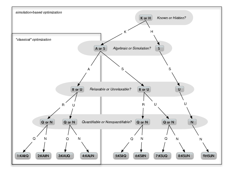
Here we provide examples for each of the nine leaves of the constraint taxonomy tree:

For additional information, and to submit use cases, please contact the authors.

Short case studies

This supplement shows that each of the nine leaves of the taxonomy tree is nonempty by providing constraint specifications, including examples from the literature, that belong to each leaf.

We note that many SBO problem specifications in the literature are composed of constraints of different types. The community groundwater problem [5] has KSRQ constraints as well as bound and linear constraints (KA**), while the LOCKWOOD problem [12] has a linear objective and simulation constraints (S); different simulation-based instances of the LOCKWOOD constraints are considered in [7] alongside solution methodologies for the resulting formulations. The STYRENE problem from [2] has 11 simulation constraints corresponding to Leaves 5 and 8 of the taxonomy tree: 7 quantifiable and relaxable constraints KSRQ, and 4 unrelaxable binary constraints KSUN.

0.1 KARQ: Quantifiable Relaxable Algebraic Known

This constraint class captures the most common types of constraints found in classical nonlinear optimization.

Ex.-

location₁ forest

The GMON problem described in [1] involves placing gamma monitoring devices in a region represented by the image of a map. There are several locations on the map (corresponding to forests, lakes, etc.) that are deemed unallowable for placement. However, the simulation, which analyzes the effects of placing devices at particular locations, is independent of the surface topology and thus can still evaluate such unallowable placements. The constraints associated with these unallowable locations are also quantifiable, since one can compute distances to the nearest (in)feasible location on the map.

Ex.-

0.15 ≤ x₁ ≤ 0.17

In [8], a nonlinear-least-squares problem is solved for parameter values that calibrate a nuclear energy density functional to experimental data. Each residual involves running a simulation associated with self-consistency of the underlying system. Bounds are imposed in [8] on half of the parameters (those associated with nuclear matter properties) because the unconstrained solution yields values that are not transferable to other nuclear structure calculations. Because the simulation still yields meaningful output when these bounds are violated (as evidenced by the unconstrained problem being solved), these algebraic and quantifiable constraints are also relaxable.

Ex.-

x₁ ∈{0,1}

A violation measure is quantified by, for example, min|x_i|, |1−x_i| and thus this constraint is KARQ provided the binary variable x₁ is relaxable.

0.2 KARN: Nonquantifiable Relaxable Algebraic Known

A good example of an KARN constraint is a categorical (e.g., nonordinal) variable constrained to a subset of its possible values. Such cases arise often in multifidelity optimization.

Ex.-

simulator = Cart3D

For the purpose of designing a supersonic airfoil, [10] considers different available analysis simulators – such as a linearized panel method (“panel”) and an Euler CFD solver (“Cart3D”) – with varying fidelity levels. The final design must be evaluated by the more costly and accurate Cart3D simulator, but an optimization algorithm can use the less expensive, inaccurate panel simulator at intermediate points. The constraint “simulator = Cart3D” is relaxable because another option for the simulator exists.

Ex.-

x₂ = O2 if x₁ = gcc

Consider a simulator that drives a C++ compilation, based on two categorical variables, each specified to take on two allowable values, x₁ ∈ {gcc,icc} and x₂ ∈ {O2,O3}. We want the final solution to have x₂ = O2 if x₁ = gcc, and this constraint is of type KARN.

We note that the two set constraints, x₁ ∈{gcc,icc} and x₂ ∈{O2,O3}, may be KAUN; see below.

0.3 KAUQ: Quantifiable Unrelaxable Algebraic Known

In SBO, one of the most common occurrences of KAUQ constraints are algebraic constraints that play a (possibly secondary) role of ensuring that the input to a simulation satisfies the expectations of the simulator.

Ex.-

r_i ≥ 0, i = 1,…6

For the groundwater bioremediation problem considered in [7], pumping rates r must be determined for each of six extraction wells. Because the simulator was hardcoded to allow only for extraction (and not injection) at these six sites, the constraints are unrelaxable. Furthermore, the quantity max{0,r_i} provides a quantifiable measure of feasibility.

Ex.-

x ∈{1,3,4} (or x belonging in any set with a means of measuring distance to the set)

When this constraint is unrelaxable, it is a KAUQ constraint; the distance to the set provides a means of quantifying how infeasible an x is (despite that one could not evaluate some simulation quantity at such infeasible points).

0.4 KAUN: Nonquantifiable Unrelaxable Algebraic Known

The allowable domain of a categorical variable is a typical example of a KAUN constraint.

Ex.-

compiler ∈{gcc,icc}

Categorical decision variables often exist when optimizing the performance of a computer code. For example, for optimization of linear algebra kernels in [4], categorical variables such as loop order (e.g., permuting groups of nested for loops) and compiler type are considered.

0.5 KSRQ: Quantifiable Relaxable Simulation Known

Any quantifiable and relaxable constraint that depends on a simulation output is a KSRQ constraint.

Ex.-

Minimal purity level of produced styrene of 0.99.

In the chemical engineering application for the production of styrene considered in [2], called STYRENE, one of the simulation outputs is the purity of the styrene produced. The problem demands that a minimal purity level is met, but intermediate designs can fall below this level, with a natural measure of violation being how far short of 0.99 the obtained purity level is.

Ex.-

Percentage of test problems solved must be at least 90%.

In [3], the algorithmic parameters of an optimization solver are tuned in order to minimize the CPU time needed to solve a set of test problems. Here, the “simulator” is a call of the solver being tuned on a particular test problem. The authors consider constraints on correctness of the output, in particular that at least 90% of the runs satisfy a prescribed convergence criterion.

Ex.-

A budget based on economical criteria, S(x) ≤ b.

0.6 KSRN: Nonquantifiable Relaxable Simulation Known

A relaxable constraint that relies on binary or nonordinal output from a simulation is a KSRN constraint.

Ex.-

no compiler warnings

A common objective in code performance optimization is to minimize the run time of a generated code. Changes to the code may result in code that still compiles and runs, but for which undesirable warnings are produced during compilation. In [6], the run times of decision variable values that resulted in problems (errors or warnings) during compilation were discarded from the analysis. The constraint that there are no warnings requires one to generate, compile, and check the compilation output of the associated code is thus “simulation-based;” [6] only considers the binary measures of this constraint, which is relaxable since run times can still be obtained (assuming that no compile errors were seen).

Ex.-

toxicity value exceeded

A simulator displays a flag indicating whether a toxicity level has been reached during the simulation, but we know neither when this occurred nor the level of toxicity.

0.7 KSUQ: Quantifiable Unrelaxable Simulation Known

Constraints that are both quantifiable and unrelaxable arise, for example, in multidisciplinary optimization (MDO), where one has a compatibility constraint between the simulations of two or more disciplines. Violating such a constraint can lead to unmeaningful output with respect to one of the disciplines.

Ex.-

s₁ ≥ 0

Compatibility constraints in MDO often arise when a given discipline’s output(s) is used as the input of another discipline. Bounds on these quantities are typical KSUQ constraints, such as the problem presented in [11, Section 5.1]. In this example, the first discipline output (y₁) appears with a squared root in the equation of the other discipline. The bound constraint y₁ ≥ 3.16 is specified in [11] and is a KSRQ constraint because it can be relaxed (albeit not arbitrarily so) and still result in meaningful output from the second discipline. The constraint y₁ ≥ 0, however, is unrelaxable and thus a KSUQ constraint (despite seeming to be redundant in the presence of the relaxable constraint y₁ ≥ 3.16).

Ex.-

c_S(x) ≥ 0

One of the outputs c_S(x) of a simulation is a concentration level; if it is below zero, the simulation stops and displays NaN for all the outputs except c_S. Consequently, this constraint is both unrelaxable and quantifiable (since there is a measure for how close one is to violating this constraint).

0.8 KSUN: Nonquantifiable Unrelaxable Simulation Known

Constraints based on binary- and nonordinal-valued simulation outputs that must be satisfied are typical KSUN constraints.

Ex.-

SEP-STY is structurally acceptable for subsequent simulations.

In the STYRENE problem of [2], four of the eleven simulation-based constraints correspond to binary flags about the convergence of internal numerical methods. In the case of the SEP-STY flag denoting failure, some of the other flags may still denote success; hence, one has richer information about the source of failure than one does for a hidden constraint.

Ex.-

exitflag = 0

If a simulation outputs an exit flag that denotes success (“0”) or multiple error code values, each with associated documentation, then one can have an indication for why the simulation did not succeed.

Each of these examples is not a hidden constraint since the reason for the violation can be identified. In contrast, a single binary flag indicating that the simulation failed is considered as a hidden constraint. In the same way, an error message that cannot be interpreted is equivalent to such a flag and hence should be interpreted as hidden.

0.9 HSUN: Hidden

Hidden constraints provide no information about the cause for failure of a simulation.

Ex.-

When sampled uniformly from a specified hyperrectangle, the STYRENE black box of [2] terminates prematurely 60% of the time, resulting in a failure. These failures are not related to the four binary flags described in the KSUN examples and thus one has no means of targeting the cause of the failure.

Ex.-

The simulation failed to complete and nothing is displayed, or a simple flag is raised or an undocumented error number indicated.

References